Google TurboQuant: 3-Bit KV Cache With Zero Accuracy Loss

A post on the Google Research blog yesterday (March 25) rattled the semiconductor industry. The technique is called TurboQuant — a KV cache compression method that claims 6x memory reduction, 8x attention computation speedup, and zero accuracy loss. My first reaction, honestly, was “yet another cherry-picked benchmark.”

Then I read the paper. The math is cleaner than I expected, and TechCrunch even ran a piece comparing it to Pied Piper from Silicon Valley. With a presentation scheduled at ICLR 2026, academic peer review is coming soon. Today I want to break down how this technique actually works and what it means for LLM inference costs.

Why KV Cache Is a Problem

In LLM inference, the biggest memory bottleneck isn’t model weights — it’s the KV cache. The Transformer attention mechanism has to store the Key and Value vectors for every preceding token. The longer the context, the more the cache grows, linearly.

Some concrete numbers:

• For a Llama 3.1 405B model with a 128K context window, the KV cache alone consumes tens of gigabytes
• After loading the model itself onto an H100 with 80GB VRAM, there’s barely room left for the cache
• Increasing batch size to boost throughput is constrained by this same memory pressure

There have been plenty of attempts to solve this with quantization. INT8 and INT4 are the standard approaches, but going below 3 bits has historically meant a noticeable drop in accuracy — that’s been the hard limit.

TurboQuant’s Two Core Ideas

TurboQuant combines two independent techniques.

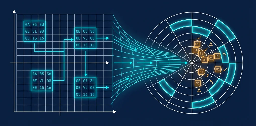
1. PolarQuant — Eliminating Normalization via Polar Coordinates

Standard quantization normalizes a vector first, then applies scalar quantization. The problem: you have to store the norm separately, and error accumulates across that process.

PolarQuant flips the idea. Instead of working in Cartesian coordinates, it transforms vectors into polar coordinates. In polar form, direction (angle) and magnitude (radius) are naturally separated, so the normalization step becomes unnecessary. You only need to uniformly quantize the angular components, which substantially reduces error.

I find this approach genuinely clever. Rather than solving the quantization problem with a better quantization algorithm, it changes the coordinate system to make the problem easier in the first place.

2. QJL — Bias Correction with 1-Bit Signs

The second enemy of quantization is bias. When computing dot products between quantized vectors, systematic error accumulates — ignore it, and your attention scores drift.

QJL (Quantized Johnson-Lindenstrauss) applies a dimensionality reduction technique called the JL transform to eliminate quantization bias using 1-bit sign correction. The additional memory overhead is minimal, and the computational cost is reportedly negligible.

# Conceptual pseudocode — refer to the paper for the actual implementation
def turboquant_attention(Q, K, V):
    # 1. Convert Key/Value to polar coordinates, then 3-bit quantize
    K_polar = to_polar(K)
    K_quant = uniform_quantize(K_polar.angles, bits=3)

    # 2. Generate QJL 1-bit sign correction
    sign_correction = qjl_sign_bits(K, Q)

    # 3. Compute corrected attention scores
    scores = corrected_dot_product(Q, K_quant, sign_correction)
    return softmax(scores) @ quantize(V, bits=3)

Performance by the Numbers

Metric	FP16 (Baseline)	TurboQuant (3-bit)	Improvement
KV Cache Memory	Baseline	1/6	6x reduction
Attention Speed	Baseline	8x	On H100
Accuracy (perplexity)	Baseline	Identical	No loss
Model Retraining	—	Not required	Drop-in

The “no retraining required” point is particularly important. This is a drop-in replacement — it can be applied to already-deployed systems as-is.

Honest Skepticism

That said, I do have questions. A few worth raising:

First, it’s not yet clear that “zero accuracy loss” holds across all tasks. The paper demonstrates this on perplexity benchmarks, but whether the same quality is maintained for long-form generation or complex reasoning tasks requires independent validation. It’ll be worth watching what additional experiments the ICLR reviewers ask for.

Second, implementation complexity in real production environments is unclear. Performing polar coordinate transforms and QJL sign correction in real time will likely require custom CUDA kernels — and whether those can be straightforwardly integrated into frameworks like vLLM or TensorRT-LLM is a separate question entirely.

Third, the market’s reaction to memory semiconductor stocks seems overblown. There were reports of a modest drop in memory chip stocks following the TurboQuant news, and frankly, that’s an overreaction. For KV cache memory savings to meaningfully reduce HBM demand, every major inference framework would need to adopt this technique — and that realistically takes one to two years at minimum.

Why It’s Still Worth Paying Attention To

Despite those critiques, I think the direction of this research has real value.

A significant portion of LLM inference costs comes from GPU memory. Model weights are already being compressed through various quantization schemes (GPTQ, AWQ, GGUF, etc.), but KV cache has largely been left untouched. What TurboQuant demonstrates is a path to handling long contexts efficiently without scaling hardware.

The scenario I’m most excited about is local LLMs. Running a 128K context on a consumer GPU with 24GB VRAM is currently near-impossible — but if you can cut KV cache by 6x, that changes the picture entirely. If the llama.cpp ecosystem picks this up, things get very interesting very fast.

References

• TurboQuant: Redefining AI efficiency with extreme compression — Google Research Blog
• Google TurboQuant AI Memory Compression — TechCrunch
• Google’s TurboQuant compresses LLM KV caches to 3 bits — Tom’s Hardware
• Google’s new TurboQuant algorithm speeds up AI memory 8x — VentureBeat